ML/사이킷런
사이킷런을 이용한 붓꽃 데이터 분류(Classification)
야뤼송
2023. 12. 29. 14:28
반응형
사이킷런에서는 여러 예제를 제공하고 있는데 그 중 많이 사용되는 것이 붓꽃 데이터를 이용하여 품종을 분류할 수 있다.
붓꽃 데이터 세트에서 꽃잎의 길이와 너비, 꽃받침의 길이와 너비 4개의 feature를 기반으로 품종을 예측할 수 있다.
1. 붓꽃 품종 예측 프로세스
- 데이터 세트 분리 : 데이터를 학습 데이터와 테스트 데이터로 분리
- 모델 학습 : 학습 데이터를 기반으로 ML 알고리즘을 적용하여 모델 학습
- 예측 수행 : 학습된 ML 모델을 이용해 텟흐트 데이터의 분류를 예측
- 평가 : 이렇게 예측된 결과값과 테스트 데이터의 실제 결과값을 비교하여 ML 모델의 성능을 평가
2. 실습 - 데이터 세트 분리
제공되는 붓꽃 데이터는 다음과 같이 구성되어 있다.
- 타켓 데이터 : setosa, versicolor, virginica 이렇게 3가지의 붓꽃종
- 특징(feature) 데이터
- 꽃받침 길이(Sepal Length)
- 꽃받침 폭(Sepal Width)
- 꽃잎 길이(Petal Length)
- 꽃잎 폭(Petal Width)
실습을 위해 사이킷런의 필요 모듈을 로딩하고 데이터 세트를 가져온다.
import pandas as pd

# 붓꽃 데이터 세트를 로딩합니다.
iris = load_iris()

print(iris.DESCR) # Description 속성을 이용해서 데이터셋의 정보를 확인
.. _iris_dataset:

Iris plants dataset
--------------------

**Data Set Characteristics:**

    :Number of Instances: 150 (50 in each of three classes)
    :Number of Attributes: 4 numeric, predictive attributes and the class
    :Attribute Information:
        - sepal length in cm
        - sepal width in cm
        - petal length in cm
        - petal width in cm
        - class:
                - Iris-Setosa
                - Iris-Versicolour
                - Iris-Virginica

    :Summary Statistics:

    ============== ==== ==== ======= ===== ====================
                    Min  Max   Mean    SD   Class Correlation
    ============== ==== ==== ======= ===== ====================
    sepal length:   4.3  7.9   5.84   0.83    0.7826
    sepal width:    2.0  4.4   3.05   0.43   -0.4194
    petal length:   1.0  6.9   3.76   1.76    0.9490  (high!)
    petal width:    0.1  2.5   1.20   0.76    0.9565  (high!)
    ============== ==== ==== ======= ===== ====================

    :Missing Attribute Values: None
    :Class Distribution: 33.3% for each of 3 classes.
    :Creator: R.A. Fisher
    :Donor: Michael Marshall (MARSHALL%PLU@io.arc.nasa.gov)
    :Date: July, 1988

The famous Iris database, first used by Sir R.A. Fisher. The dataset is taken
from Fisher's paper. Note that it's the same as in R, but not as in the UCI
Machine Learning Repository, which has two wrong data points.

This is perhaps the best known database to be found in the
pattern recognition literature.  Fisher's paper is a classic in the field and
is referenced frequently to this day.  (See Duda & Hart, for example.)  The
data set contains 3 classes of 50 instances each, where each class refers to a
type of iris plant.  One class is linearly separable from the other 2; the
latter are NOT linearly separable from each other.

.. topic:: References

   - Fisher, R.A. "The use of multiple measurements in taxonomic problems"
     Annual Eugenics, 7, Part II, 179-188 (1936); also in "Contributions to
     Mathematical Statistics" (John Wiley, NY, 1950).
   - Duda, R.O., & Hart, P.E. (1973) Pattern Classification and Scene Analysis.
     (Q327.D83) John Wiley & Sons.  ISBN 0-471-22361-1.  See page 218.
   - Dasarathy, B.V. (1980) "Nosing Around the Neighborhood: A New System
     Structure and Classification Rule for Recognition in Partially Exposed
     Environments".  IEEE Transactions on Pattern Analysis and Machine
     Intelligence, Vol. PAMI-2, No. 1, 67-71.
   - Gates, G.W. (1972) "The Reduced Nearest Neighbor Rule".  IEEE Transactions
     on Information Theory, May 1972, 431-433.
   - See also: 1988 MLC Proceedings, 54-64.  Cheeseman et al"s AUTOCLASS II
     conceptual clustering system finds 3 classes in the data.
   - Many, many more ...
iris 데이터 세트에서 피처 데이터와 레이블 데이터로 각각 분리한다.
# iris.data는 iris 데이터 세트에서 피처(feature)만으로 된 데이터를 numpy로 가지고 있다.
iris_data = iris.data

# iris.target은 붓꽃 데이터 세트에서 레이블(결정 값) 데이터를 numpy로 가지고 있다.
iris_label = iris.target
붓꽃 데이터 세트를 자세히 보기 위해 피처와 레이블 데이터를 통해 DataFrame으로 변환한다. 변환된 데이터의 라벨 값에서 0은 setosa , 1은 versicolor, 2는 virginica이다.
# pandas를 이용한 DataFrame으로 변환
iris_df = pd.DataFrame(data=iris_data, columns=iris.feature_names)
iris_df['label'] = iris.target
iris_df.head(3)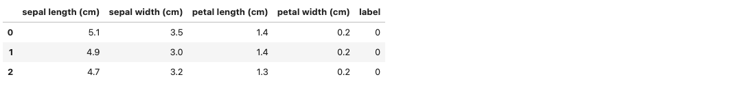
학습 데이터와 테스트 데이터 세트로 분리한다.
X_train, X_test, y_train, y_test =
train_test_split(iris_data, iris_label, test_size=0.2, random_state=11)
위의 코드를 하나 하나 확인해보면 다음과 같다.
- X_train : 학습용 Feature 데이터 셋
- X_test : 테스트용 Feature 데이터 셋
- y_train : 학습용 target 값
- y_test : 테스트용 target 값
(보통 대문자 X는 Feature를 뜻하고 소문자 y는 target을 의미한다) - test_size
- 전체 데이터 중 얼마큼을 테스트 데이터로 만들지를 결정하는 파라미터
- test_size = 0.2 인 경우 80% train, 20% test 데이터 세트를 추출 - random_state :
- 호출할 때마다 동일한 학습/테스트용 데이터 세트를 생성하기 위해 주어지는 난수 값.
- train_test_split는 랜덤으로 데이터를 분리하므로 train_test_split를 설정하지 않으면 수행할 때마다 다른 학습/테스트 데이터 세트가 생성된다. 따라서 random_state를 설정하여 수행 시 결과값을 동일하게 맞춰준다.
가령 1~ 100까지 일련번호로 된 100개의 데이터를 train_test_split(.., test_size=0.2) 로 수행하면 해당 함수를 첫번째 수행할 때는 1~80 번이 train, 81~100번이 test가 될 수 있지만, 다시 수행하면 이번에 21~100번이 train, 1~20번이 test가 될 수 있다. 80%, 20% 로 나누는건 동일하지만 함수를 수행 시마다 추출한 레코드들을 달라질수 있다.
내부적으로 80%, 20% 로 나눌때 random 함수를 적용한다.
random_state=1 이라고 하면 바로 이 random 함수의 seed 값을 고정시키기 때문에 여러번 수행하더라도 같은 레코드를 추출하게 된다. 이때 random_state에는 어떤 숫자를 적든 그 기능은 같기 때문에 어떤 숫자를 적든 상관없다.
3. 실습 - 학습데이터 세트로 학습(Train) 수행
# DecisionTreeClassifier 객체 생성
dt_clf = DecisionTreeClassifier(random_state=11)

# 학습 수행 *
# 학습 수행을 위해 학습용 feature 데이터 셋과 학습용 target 값을 사용한다.
dt_clf.fit(X_train, y_train)
fit() 함수는 학습을 수행하기 위한 메소드이다.
4. 실습 - 테스트 데이터 세트로 예측(Predict) 수행
# 학습이 완료된 DecisionTreeClassifier 객체에서 테스트 데이터 세트로 예측 수행.
pred = dt_clf.predict(X_test)
pred
array([2, 2, 1, 1, 2, 0, 1, 0, 0, 1, 1, 1, 1, 2, 2, 0, 2, 1, 2, 2, 1, 0, 0, 1, 0, 0, 2, 1, 0, 1])
5. 실습 - 예측 정확도 평가
에측 정확도를 평가하기 위해서는 accuracy_score을 사용한다.
accuracy_score에 정답배열과 예측배열을 넣으면 정확도가 평가된다.
from sklearn.metrics import accuracy_score
print('예측 정확도: {0:.4f}'.format(accuracy_score(y_test,pred)))
예측 정확도: 0.9333
우리가 수행한 품종 분류 정확도를 평가하기 위해 정답 배열인 y_test와 예측을 수행한 pred 배열을 입력하면 0.9333 이라는 정확도 값을 얻을 수 있다.
반응형